Master Conditional Formatting Rows Based on Cell Values in Google Sheets

Introduction

Mastering the art of data visualization can significantly change how we interpret information. Google Sheets stands out as a powerful tool for achieving this, particularly through its conditional formatting feature. This capability allows users to dynamically alter the appearance of rows based on specific cell values. As a result, identifying trends, errors, and critical data points becomes much easier at a glance.

However, many users face challenges when it comes to effectively applying these techniques. Common pitfalls can hinder their analysis, leaving them frustrated and overwhelmed. So, how can you harness the full potential of conditional formatting? By mastering this feature, you can enhance your spreadsheet functionality and streamline decision-making, ultimately leading to more informed choices.

Understand Conditional Formatting in Google Sheets

In Google Sheets, the feature of conditional formatting row based on cell empowers users to automatically modify the appearance of cells according to specific criteria. This feature is invaluable for highlighting trends, pinpointing errors, and visually organizing data. Here are the key aspects to understand:

Dynamic Formatting: Conditional formatting alters the cell's background color, text color, or style depending on the values within the cell or related cells.
Rules and Conditions: Users can set guidelines such as 'greater than', 'less than', or 'equal to' to create conditional formatting row based on cell, which dictates when styling is applied.
Visual Impact: By employing color coding and styles, users can swiftly identify crucial data points, enhancing the readability and analysis of spreadsheets.

Grasping these foundational concepts is essential, as it equips users to implement these strategies effectively in practical scenarios throughout this guide.

The center represents the main topic, and the branches show key aspects of conditional formatting. Each color-coded branch helps you quickly identify different areas of focus related to the main concept.

Apply Conditional Formatting Based on Cell Values

Mastering Conditional Formatting in Google Sheets
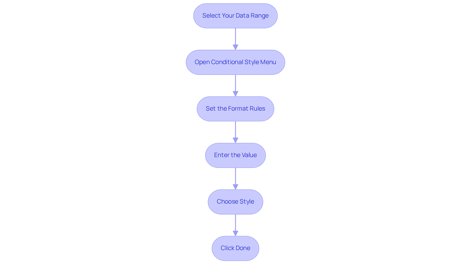
To enhance the readability of your spreadsheets, applying conditional formatting based on cell values is essential. Here’s how you can do it effectively:

Select Your Data Range: Click and drag to highlight the areas you want to format.
Open Conditional Style Menu: Navigate to the top menu, click on Format, and select Conditional style.
Set the Format Rules: In the sidebar that appears, choose the type of rule you want to apply. For instance, select 'Format items if...' and choose a condition such as 'Greater than'.
Enter the Value: Input the value that will activate the style. For example, to highlight cells greater than 100, enter 100.
Choose Style: Select the style you wish to apply, such as background color or text color.
Click Done: After establishing your rules and styles, click Done to apply the design.

By following these steps, you can effectively use conditional formatting row based on cell to highlight critical information points that meet specific criteria. This not only enhances the readability of your spreadsheets but also streamlines your analysis process. In fact, finance experts have observed that using conditional styles can save an average of 30% of their time spent on analysis, enabling quicker decision-making and deeper insights.

As industry specialists note, "Conditional styling is a game changer for information analysis, allowing us to visualize trends and make informed decisions quickly." To maximize the benefits of this powerful tool, regularly assess and modify your styling guidelines to ensure they align with evolving information needs. This proactive approach will significantly enhance your efficiency and effectiveness in data analysis.

Each box represents a step in the process of applying conditional formatting. Follow the arrows to see how to move from one step to the next, ensuring you don't miss any important actions.

Explore Examples of Conditional Formatting Applications

The use of conditional formatting row based on cell in Google Sheets provides powerful tools for enhancing data visibility and monitoring key metrics. Here are some practical applications:

Sales Performance Tracking: Highlight cells in a sales report that exceed targets. For instance, if a sales figure in column B surpasses $10,000, format that cell with a green background to signify success. This method provides immediate visual feedback through conditional formatting row based on cell, which also aids in quick decision-making. Case studies reveal that businesses improved sales strategies through effective KPI tracking. A local chain of hobby, book, and music shops, for example, employed situational styling to recognize sales patterns, resulting in a strategic shift that enhanced their market performance.
Budget Oversight: Utilize rule-based highlighting to indicate costs that exceed allocated amounts. If an entry in the expenses column surpasses the related budget entry, use conditional formatting row based on cell to apply a red text color to alert users. This technique, utilizing conditional formatting row based on cell, has proven beneficial in various organizations by allowing for swift adjustments to spending and enhancing overall financial oversight. A travel company implemented conditional styling to monitor operational costs, helping them address inefficiencies and improve customer satisfaction scores.
Deadline Reminders: In project management sheets, format cells in a deadline column to turn yellow if the date is approaching (e.g., within 7 days). This visual cue assists teams in prioritizing tasks effectively, ensuring that critical deadlines are met and resources are allocated efficiently. As noted by a Content Strategist at Zaver.one, effective structuring techniques can enhance performance analysis and enable faster, data-informed decisions.

These examples illustrate the adaptability of flexible styles, empowering users to utilize conditional formatting row based on cell for improved information interpretation and operational effectiveness. By leveraging these techniques, finance professionals can transform raw data into actionable insights, ultimately driving better business outcomes.

The central node represents the main topic, while the branches show different applications of conditional formatting. Each sub-branch provides details on how these techniques can improve data visibility and decision-making.

Troubleshoot Common Conditional Formatting Issues

When using conditional styles in Google Sheets, users often face common challenges. Here’s how to troubleshoot them effectively:

Formatting Not Applying: First, verify that the selected range for formatting matches the intended cells. An incorrect range will prevent the styling from being applied. Ensuring the correct range is set in the 'Apply to range' field is essential for successful presentation.
Conflicting Rules: Google Sheets processes multiple rules in a specific order. If a rule seems ineffective, check for any overriding rules. Adjust the sequence of guidelines in the rule sidebar to resolve conflicts. Remember, users can apply up to 19 different rules within single-color conditional styles, offering flexibility in managing these issues.
Formula Errors: For those using custom formulas, accuracy is key. A common mistake is neglecting absolute references when necessary. Review your formulas carefully to avoid errors. As Robert A. Lee, Senior Editor, notes, "Natural language inquiries in Sheets increased by 44% in enterprise environments," highlighting the importance of precise formula application in enhancing analysis.
Type Mismatch: Ensure that the types in the boxes align with the conditions outlined in the style guidelines. For instance, when comparing numbers, confirm that the cells are formatted as numbers rather than text. This alignment is crucial for effective information visualization, as context-specific styling is a powerful tool for improving spreadsheet analysis.

Addressing these frequent problems can significantly enhance the efficiency of situational styling, particularly through the use of conditional formatting row based on cell, empowering users to leverage this powerful tool for superior data visualization and analysis. Statistics reveal that a substantial percentage of users encounter issues with conditional formatting rules, underscoring the importance of these troubleshooting steps.

Follow the arrows to identify common issues with conditional formatting and see the steps to resolve them. Each box represents a specific problem, and the sub-points provide actionable solutions.

Conclusion

Mastering conditional formatting in Google Sheets is essential for enhancing data visibility and streamlining analysis. By automatically adjusting cell styles based on specific criteria, this powerful tool enables quick identification of critical information and facilitates informed decision-making through effective data visualization.

The article outlines essential steps for applying conditional formatting:

Selecting data ranges
Setting format rules
Troubleshooting common issues

Key applications, such as tracking sales performance, monitoring budgets, and managing project deadlines, showcase how conditional formatting can transform raw data into actionable insights. Furthermore, the importance of regularly updating formatting rules to align with evolving data needs is emphasized, reinforcing the value of this feature.

Embracing conditional formatting in Google Sheets transcends mere aesthetic improvements; it represents a strategic approach to data management that can significantly enhance operational efficiency. By implementing the techniques and best practices discussed, users can unlock the full potential of their spreadsheets, leading to better analysis and ultimately driving improved business outcomes.

Frequently Asked Questions

What is conditional formatting in Google Sheets?

Conditional formatting in Google Sheets is a feature that allows users to automatically change the appearance of cells based on specific criteria, helping to highlight trends, errors, and organize data visually.

How does dynamic formatting work in Google Sheets?

Dynamic formatting changes the background color, text color, or style of a cell depending on the values within that cell or related cells.

What types of rules can be set for conditional formatting?

Users can set rules such as 'greater than', 'less than', or 'equal to' to determine when the conditional formatting is applied to a cell.

What is the visual impact of using conditional formatting?

Conditional formatting enhances the readability and analysis of spreadsheets by using color coding and styles to help users quickly identify important data points.

Why is it important to understand the foundational concepts of conditional formatting?

Understanding the foundational concepts of conditional formatting equips users to implement these strategies effectively in practical scenarios within Google Sheets.