Master Conditional Formatting: Use a Formula to Format Cells in Sheets

Introduction

Conditional formatting in Google Sheets is an essential tool for enhancing data visibility and analysis. It allows users to automatically adjust cell appearances based on defined criteria, making it easier to interpret complex datasets. By mastering the use of formulas within this framework, individuals can harness powerful techniques that streamline data management and highlight critical information.

However, as users explore this feature, they often encounter challenges: How can one effectively create and manage these formulas to maximize their impact? This guide will delve into the nuances of conditional formatting, offering insights and practical examples designed to elevate your spreadsheet functionality. Get ready to transform your data management approach and unlock the full potential of Google Sheets.

Understand Conditional Formatting Basics

Conditional styling in Google Sheets is a powerful tool that allows users to automatically change the appearance of entries based on specific criteria. This feature is essential for highlighting important data, identifying trends, and flagging errors. Understanding the following key concepts will prepare you to leverage this functionality effectively:

Rules: Conditional formatting operates on rules that dictate when a cell's format should change. For example, you might want to emphasize cells containing values that exceed a certain threshold.
Scope: This refers to the range of cells that the styling guidelines will apply to. You can choose to format a single cell, an entire row, a column, or even the whole sheet.
Formatting Options: You have the flexibility to alter text color, background color, font style, and more, depending on the conditions you establish.

By mastering these fundamentals, you will be well-equipped to create effective rules that incorporate how to use a formula to determine which cells to format, enhancing the clarity and impact of your spreadsheets.

The center shows the main topic of conditional formatting, while the branches represent key concepts. Each branch provides specific details that help you understand how to use conditional formatting effectively.

Create a Formula for Conditional Formatting

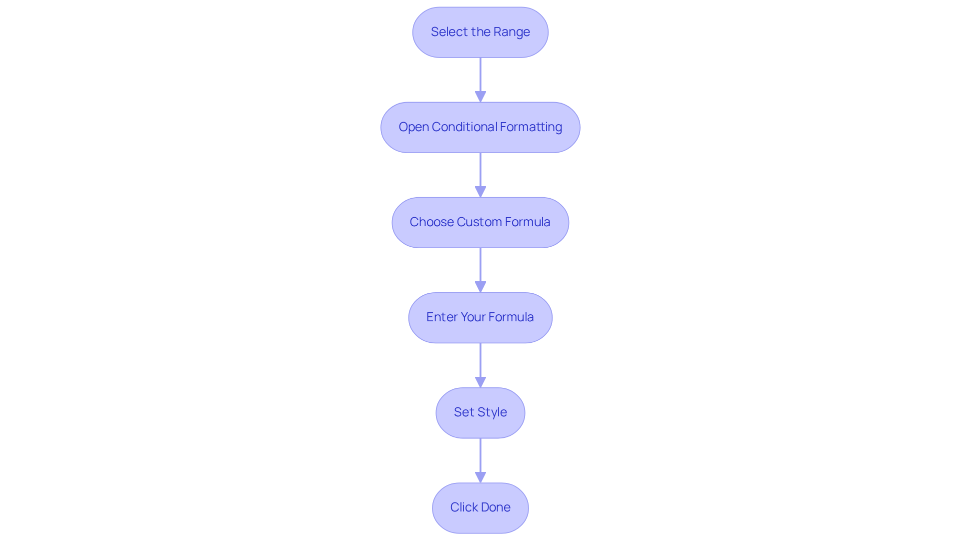
To create a formula for conditional formatting in Google Sheets, follow these essential steps:

Select the Range: Highlight the cells you want to format.
Open Conditional Formatting: Navigate to the menu, click on Format, and select Conditional formatting.
Choose Custom Formula: In the conditional format rules pane, select Custom formula is from the dropdown menu.
Enter Your Formula: Input your formula. For instance, to highlight cells in column A that are greater than 100, enter =A1>100, adjusting the cell reference as needed for your selected range.
Set Style: Choose your preferred style, such as background color or text color.
Click Done: Apply the rule by clicking Done.

Conditional styling in Google Sheets offers two primary options: Single color and Color scale. Single color applies one shade to areas meeting a specific condition, while Color scale applies a gradient based on values. By employing custom formulas, you can use a formula to determine which cells to format, allowing for the development of dynamic styles that adjust to changes in your data, significantly enhancing data analysis.

To resolve any issues with conditions in the settings, ensure that the 'Apply to range' option includes the correct cells. If you need to remove a rule for style conditions, simply click the trash bin next to the rule. Experts emphasize that this approach can lead to an average time savings of up to 30% when managing large datasets, as it streamlines the identification of key information. Companies utilizing custom conditional styles have reported enhanced data visualization, enabling quicker decision-making and more effective presentations.

Each box represents a step in the process of applying conditional formatting in Google Sheets. Follow the arrows to see how to move from one step to the next.

Apply Conditional Formatting to Common Scenarios

Conditional formatting in Google Sheets significantly enhances data analysis and visualization. Consider these practical scenarios where it can be effectively applied:

Highlighting Duplicates: To identify duplicate entries in a list, use the formula =COUNTIF(A:A, A1)>1. This highlights any entry in column A that appears more than once, ensuring data integrity and facilitating error checking.
Tracking Progress: For task lists with completion percentages, emphasize entries that are below 100% using the formula =B1<1 (assuming column B contains the percentages). This allows for quick identification of incomplete tasks, aiding in project management.
Flagging Expired Dates: To highlight dates that have passed, apply the formula =A1<TODAY(). This will format any date in column A that is earlier than today, helping users manage deadlines effectively.
Visualizing Performance: In sales data, highlight cells that exceed a target value with =B1>5000 to emphasize sales figures greater than 5000 in column B. This visual cue can drive performance discussions and strategic decisions.

These examples illustrate how situational styling simplifies data analysis, enabling finance professionals to use a formula to determine which cells to format, monitor progress, and ensure data precision. Moreover, statistics indicate that to enhance adaptability, you can use a formula to determine which cells to format in various ways. For instance, it can help identify cells with values less than 50, providing further insights into data trends. Case studies, such as "Applying Conditional Formatting in Google Sheets," showcase the practical application of these techniques, demonstrating their effectiveness in real-world scenarios. As noted by finance experts like Zakhar Yung, adaptive styling not only enhances data presentation but also aids in extracting significant insights from complex datasets.

The central node represents the main topic of conditional formatting, while the branches show different scenarios where it can be applied. Each formula under the branches provides a quick reference for how to implement the formatting.

Manage and Troubleshoot Conditional Formatting Rules

To effectively manage and troubleshoot your conditional formatting rules in Google Sheets, follow these essential guidelines:

View Current Guidelines: Access the style panel to examine all criteria applied to the selected range. This allows you to modify or remove guidelines as necessary, ensuring your formatting is always relevant.
Prioritize Guidelines: Conditional formatting guidelines are executed in the order they appear. If multiple guidelines apply to the same cell, only the first one that evaluates to TRUE will take effect. Rearrange guidelines easily by dragging them within the pane to achieve the desired outcome.
Check for Errors: If your layout isn’t functioning as intended, review your formulas for syntax errors or incorrect references. Confirm that the selected range aligns with the logic of your formulas to use a formula to determine which cells to format and avoid any issues.
Evaluate Your Guidelines: After setting your guidelines, assess their effectiveness by altering the information in the applicable sections. This will help you verify that the styles change as anticipated, enhancing the visual impact of your data.
Remove Styles: To eliminate all specific styles from a range, select the desired cells, navigate to Format, and choose Clear styles. This action helps maintain a clean and organized spreadsheet.

By effectively managing your conditional formatting rules, you can use a formula to determine which cells to format, thereby maintaining clarity and enhancing the visual impact of your spreadsheets, making them more informative and easier to analyze.

Each box represents a step in managing your conditional formatting rules. Follow the arrows to see the order in which you should apply these guidelines for effective troubleshooting.

Conclusion

Mastering conditional formatting in Google Sheets is not just a skill; it’s a game changer for anyone looking to manage data more effectively. Imagine transforming your spreadsheets into organized, visually appealing tools that highlight critical information and simplify data analysis. This is the power of conditional formatting.

In this article, we’ve explored the essential elements of conditional formatting, including:

The foundational concepts of rules
Scope
The various formatting options available

You’ve learned how to create custom formulas tailored to your specific needs - whether it’s tracking progress, identifying duplicates, or flagging expired dates. Moreover, we’ve discussed best practices for managing and troubleshooting these formatting rules, ensuring clarity and effectiveness in your spreadsheets.

By incorporating these conditional formatting techniques, you significantly enhance the usability of your data in Google Sheets. These strategies empower you to transform your spreadsheets into powerful tools for analysis and presentation. Not only do they improve data visualization, but they also foster a more efficient workflow, enabling you to make informed decisions swiftly. Implementing these advanced techniques can lead to increased productivity and a clearer understanding of complex datasets.

Now is the time to take action. Embrace these practices and elevate your data management skills. With conditional formatting, you’re not just organizing data; you’re unlocking the potential for insightful analysis and impactful decision-making.

Frequently Asked Questions

What is conditional formatting in Google Sheets?

Conditional formatting in Google Sheets is a feature that allows users to automatically change the appearance of entries based on specific criteria, helping to highlight important data, identify trends, and flag errors.

What are the key components of conditional formatting?

The key components of conditional formatting include rules, scope, and formatting options. Rules dictate when a cell's format should change, scope refers to the range of cells the formatting applies to, and formatting options allow users to alter text color, background color, font style, and more.

How do rules work in conditional formatting?

Rules in conditional formatting operate by specifying conditions that determine when a cell's format should change, such as emphasizing cells with values that exceed a certain threshold.

What does 'scope' mean in the context of conditional formatting?

Scope refers to the range of cells that the conditional formatting rules will apply to, which can include a single cell, an entire row, a column, or the whole sheet.

What formatting options are available in conditional formatting?

Formatting options in conditional formatting include changing text color, background color, font style, and other visual attributes based on the established conditions.

How can mastering conditional formatting fundamentals benefit users?

Mastering the fundamentals of conditional formatting equips users to create effective rules and use formulas to determine which cells to format, enhancing the clarity and impact of their spreadsheets.