Master Google Sheet HLOOKUP: Step-by-Step for Finance Pros

Q: What do the parameters of the HLOOKUP function mean?

- **search_key**: The value you want to find in the first row. - **range**: The scope of cells containing the data. - **index**: The row number in the range from which to return the value. - **is_sorted**: An optional parameter that indicates whether the first row is sorted; use FALSE for an exact match.

Overview

This article delves into the effective utilization of the HLOOKUP function in Google Sheets by finance professionals, focusing on its application in retrieving data from horizontal tables. It begins by outlining the function's syntax, followed by detailed, step-by-step instructions for implementation. Additionally, it addresses common errors and troubleshooting strategies, underscoring the function's pivotal role in enhancing productivity and accuracy in financial data management.

Introduction

Mastering the HLOOKUP function in Google Sheets can significantly enhance how finance professionals manage and analyze data. This powerful tool enables users to efficiently retrieve information from horizontal tables, making it indispensable in the fast-paced finance sector where accuracy and speed are crucial. Despite its advantages, many users encounter challenges such as lookup errors and formatting issues that can impede productivity.

How can finance experts effectively leverage HLOOKUP to streamline their processes while steering clear of common pitfalls?

Understand HLOOKUP: The Basics

The google sheet hlookup function is a powerful feature that enables users to search for a defined item in the first row of a selected area and return a corresponding item from a specified row within the same column. The syntax for HLOOKUP is as follows:

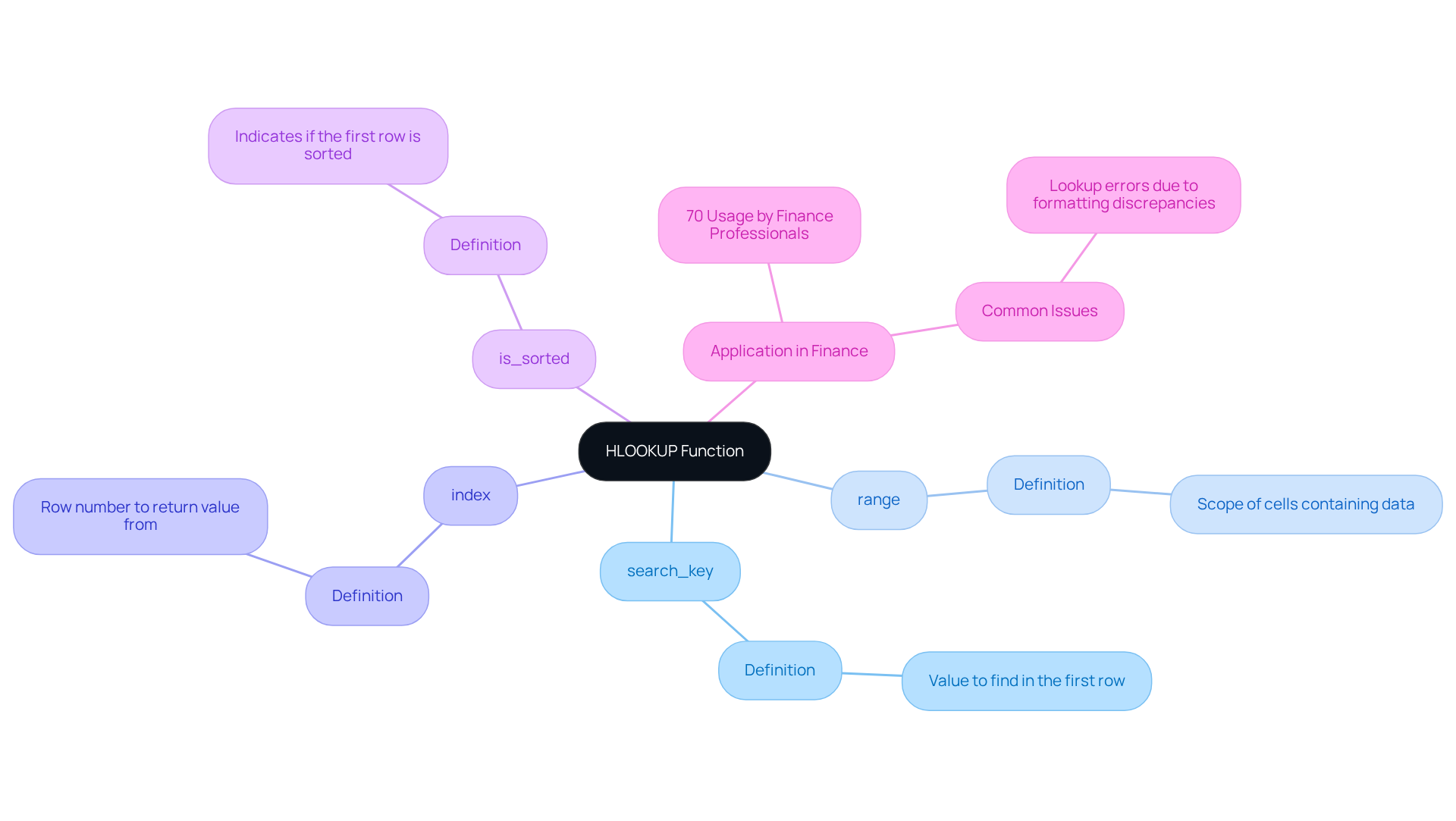
HLOOKUP(search_key, range, index, [is_sorted])

search_key: The value you want to find in the first row.
range: The scope of cells containing the data.
index: The row number in the range from which to return the value.
is_sorted: Optional. Indicates whether the first row is sorted; use FALSE for an exact match.

This function proves particularly advantageous for finance professionals, facilitating the efficient retrieval of relevant information from data organized in rows. Notably, studies indicate that approximately 70% of finance professionals utilize horizontal lookup functions in their spreadsheets, underscoring its significance in financial analysis. For instance, when examining sales data, a lookup function can swiftly extract specific metrics from a summary table, thereby streamlining the decision-making process. As Claudia Buckley, a certified Microsoft Office Expert, asserts, "The day I used my first lookup formula was the day I knew my Excel spreadsheets were more than just a convenient place to store data."

By mastering functions like google sheet hlookup, finance professionals can significantly enhance their productivity and accuracy in data management. However, users may encounter common issues, such as lookup errors where the function fails to find a value due to formatting discrepancies. Addressing these challenges is essential for leveraging the full potential of this lookup function in financial analysis.

Start at the center with the HLOOKUP function, then explore its components and see how they connect to its practical use in finance — each branch offers deeper insights into how to utilize this powerful tool.

Implement HLOOKUP in Google Sheets: Step-by-Step Instructions

To implement HLOOKUP in Google Sheets, adhere to the following steps:

Open Google Sheets: Launch Google Sheets and access the spreadsheet where you intend to utilize the function.
Select the Cell: Click on the cell designated for the result of the horizontal lookup function.
Enter the HLOOKUP Formula: Begin by typing =HLOOKUP( to initiate the function.
Input the Search Key: Enter the term you wish to search for. For example, if you are seeking 'Sales', type "Sales" or reference a cell containing the search key.
Define the Range: Specify the range of cells that encompasses the data, such as A1:D10.
Set the Index: Indicate the row number from which you wish to obtain the result. For instance, if you desire the item from the second row, type 2.
Specify the Match Type: To obtain an exact match, input FALSE. Your formula should resemble:
```
=HLOOKUP("Sales", A1:D10, 2, FALSE)
```
Press Enter: Hit Enter to execute the formula. The cell will then display the value retrieved from the specified row based on your search key.

By following these steps, you can effectively utilize the Google Sheets HLOOKUP function to extract data from horizontal tables in your financial spreadsheets.

Common Errors to Watch For

Be vigilant regarding common errors such as REF! or N/A, which may arise if the specified range is incorrect or the search key is not found. To manage #N/A errors gracefully, consider wrapping your HLOOKUP formula in the IFNA function:

=IFNA(HLOOKUP("Sales", A1:D10, 2, FALSE), "Not Found")

Using Wildcards

If you need to search for values that conform to a pattern, wildcards can be employed in your HLOOKUP function. Remember to set the last parameter, is_sorted, to FALSE when utilizing wildcards to prevent errors. For example:

=HLOOKUP("Sales*", A1:D10, 2, FALSE)

This will match any value beginning with 'Sales'. By incorporating these practices, you will enhance your data retrieval capabilities in financial spreadsheets.

Each box represents a step you need to follow. The arrows guide you through the process, and the diamonds show points where you may need to make decisions or consider alternatives, like handling errors or using wildcards.

Troubleshoot HLOOKUP Issues: Common Problems and Solutions

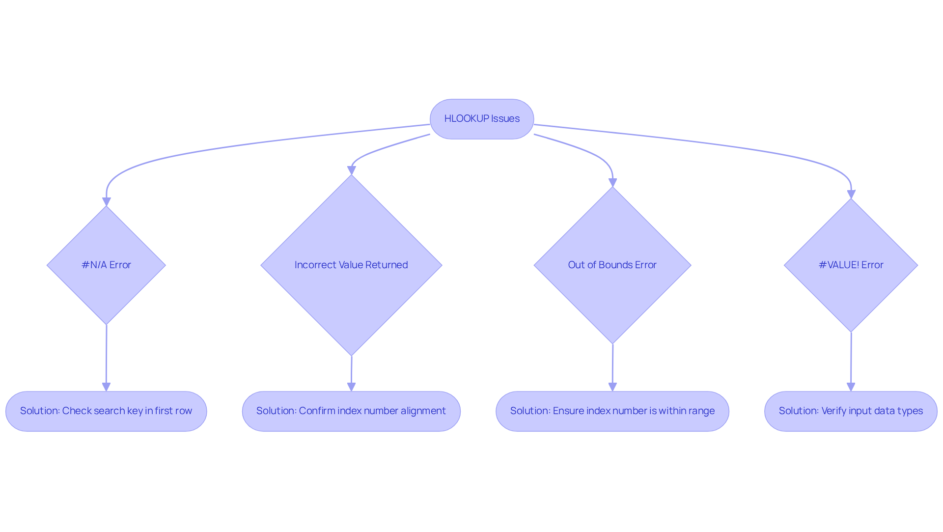
When using Google Sheets HLOOKUP, several common issues may arise. Understanding these problems and their solutions is essential for effective troubleshooting:

#N/A Error: This error indicates that the search key is not found in the first row of the specified area.
- Solution: Double-check the search key to ensure its presence in the first row.
Incorrect Value Returned: If an incorrect value is returned, it may stem from an improper index number or incorrectly set limits.
- Solution: Confirm that the index number aligns with the appropriate row in the dataset.
Out of Bounds Error: This occurs when the index number exceeds the total number of rows in the designated area.
- Solution: Ensure that the index number stays within the available range of rows.
#VALUE! Error: This error signifies an issue with the function arguments, such as mismatched data types.
- Solution: Verify that all inputs are correctly formatted and correspond to the expected data types.

By recognizing these common issues and their solutions, you can effectively troubleshoot Google Sheets HLOOKUP problems, thereby enhancing your productivity.

Each box represents a common problem you might face when using HLOOKUP, and the arrows guide you to the solutions for those problems.

Conclusion

Mastering the HLOOKUP function in Google Sheets is a transformative advantage for finance professionals, enabling swift data retrieval and enhancing analytical capabilities. This powerful tool simplifies the process of locating specific values in horizontal data arrangements and streamlines decision-making by providing quick access to essential metrics.

This guide has shared key insights on the syntax and application of HLOOKUP, including:

Detailed step-by-step instructions for implementation
Common errors to avoid
Troubleshooting tips

By understanding how to effectively utilize this function, finance experts can sidestep pitfalls such as #N/A errors and incorrect value returns, ensuring precise data management.

Embracing the HLOOKUP function can significantly elevate productivity and accuracy in financial analysis. As finance professionals navigate increasingly complex datasets, mastering tools like HLOOKUP becomes imperative. Dedicate time to practice and apply these techniques in your own spreadsheets, and witness the profound impact on how data informs your financial decisions.

Frequently Asked Questions

What is the HLOOKUP function in Google Sheets?

The HLOOKUP function is a feature that allows users to search for a defined item in the first row of a selected area and return a corresponding item from a specified row within the same column.

What is the syntax for the HLOOKUP function?

The syntax for HLOOKUP is: HLOOKUP(search_key, range, index, [is_sorted]).

What do the parameters of the HLOOKUP function mean?

search_key: The value you want to find in the first row.
range: The scope of cells containing the data.
index: The row number in the range from which to return the value.
is_sorted: An optional parameter that indicates whether the first row is sorted; use FALSE for an exact match.

Who benefits most from using the HLOOKUP function?

HLOOKUP is particularly advantageous for finance professionals, as it facilitates the efficient retrieval of relevant information from data organized in rows.

How prevalent is the use of HLOOKUP among finance professionals?

Approximately 70% of finance professionals utilize horizontal lookup functions like HLOOKUP in their spreadsheets.

Can you provide an example of how HLOOKUP is used?

For instance, when examining sales data, a lookup function can swiftly extract specific metrics from a summary table, thereby streamlining the decision-making process.

What are some common issues users may encounter with HLOOKUP?

Users may face lookup errors where the function fails to find a value due to formatting discrepancies.

Why is mastering HLOOKUP important for finance professionals?

Mastering functions like HLOOKUP can significantly enhance productivity and accuracy in data management for finance professionals.