Introduction
Mastering the SUMIF function in Google Sheets can significantly enhance how users manage data, making financial analysis not only more efficient but also more insightful. This powerful tool empowers individuals to sum values based on specific criteria, thereby streamlining reporting processes and boosting productivity. Yet, many users face challenges when implementing this function.
What are the common pitfalls?
How can they be avoided to ensure accurate results?
Understanding these aspects is crucial for leveraging the full potential of the SUMIF function.
Understand the SUMIF Function: Definition and Syntax
The SUMIF function in Google Sheets stands out as a powerful tool for summing values based on specific conditions. Its syntax is straightforward:
=SUMIF(range, criterion, [sum_range])
- range: This is the set of cells evaluated against the criterion.
- criterion: The condition that must be met for a cell to be included in the sum. This can be a number, expression, cell reference, or text.
- sum_range: This is optional. If provided, it specifies the exact cells to total; if omitted, Google Sheets sums the cells within the selected range.
For example, if you want to sum all sales exceeding $100 in a sales data range, you would write:
=SUMIF(A1:A10, ">100")
This function proves particularly beneficial for financial analysis, allowing users to quickly aggregate data based on defined criteria. Recent enhancements in Google Sheets have further improved the functionality of this formula, making it more user-friendly and efficient. In fact, a significant number of users rely on this formula for their financial analyses, underscoring its importance in data-driven decision-making. Understanding how to sumif can greatly enhance your ability to analyze financial data, streamline reporting processes, and boost overall productivity.

Implement SUMIF: Step-by-Step Instructions
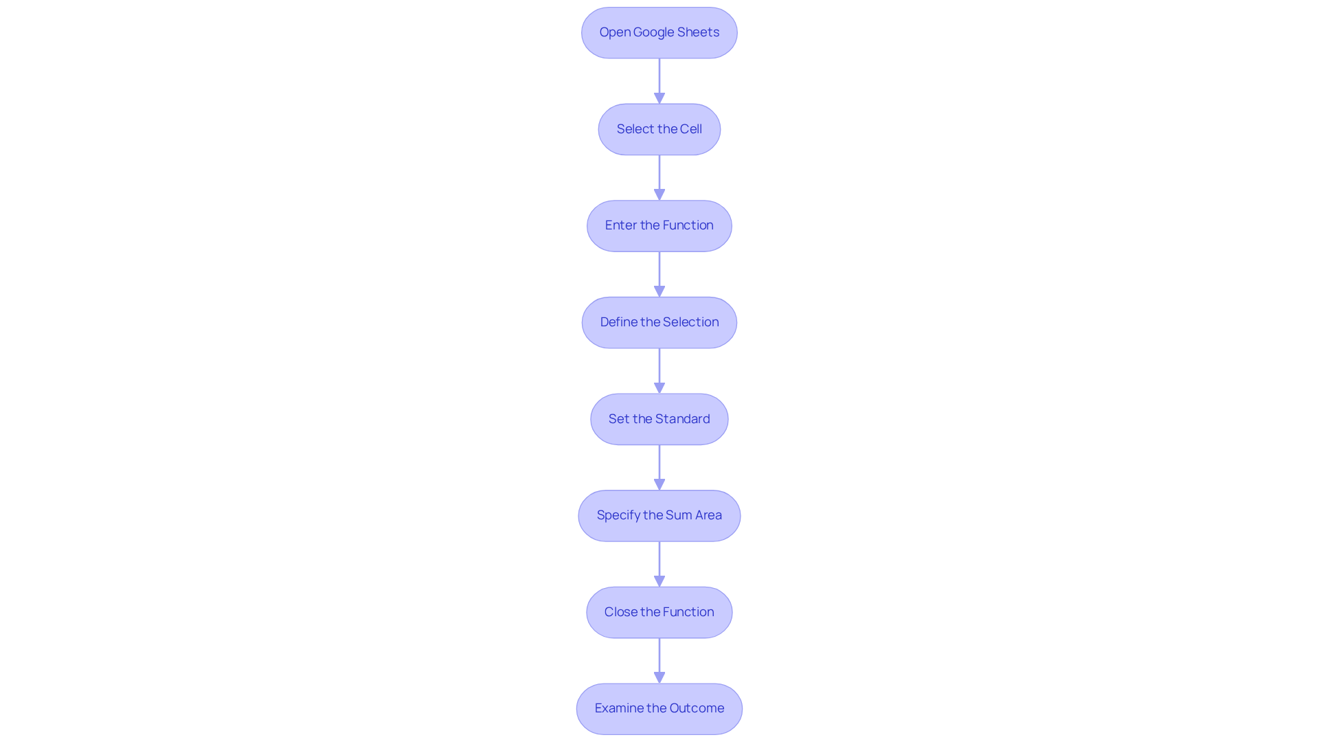
To implement the SUMIF function in Google Sheets effectively, follow these steps:
-
Open Google Sheets: Launch your Google Sheets document where you want to utilize the summation condition.
-
Select the Cell: Click on the cell where you want the outcome of the SUMIF operation to appear.
-
Enter the Function: Type
=SUMIF(to start the function. -
Define the Selection: Click and drag to choose the set of cells you wish to evaluate. For example, if your data is in cells A1 to A10, it should look like this:
=SUMIF(A1:A10,. -
Set the Standard: After the interval, type a comma and then enter your parameter. For instance, to sum values greater than 100, you would write:
=SUMIF(A1:A10, ">100",. -
Specify the Sum Area (if needed): If you wish to sum a different area, type a comma and select that area. For instance, if you wish to add values in B1 to B10 according to the conditions in A1 to A10, it would appear as follows:
=SUMIF(A1:A10, ">100", B1:B10). -
Close the Function: Type a closing parenthesis
)and press Enter. Your formula should now look like this:=SUMIF(A1:A10, ">100", B1:B10). -
Examine the Outcome: The cell will now show the total of all values in the designated sum area that satisfy the condition.
Mastering how to sumif can save finance professionals considerable time, enabling swift computations and effective data management. Avoid common mistakes such as ensuring that the range and sum range are of equal size and checking for proper formatting of criteria. Practical uses of this formula encompass monitoring expenses, evaluating sales data, and compiling financial reports.

Troubleshoot Common SUMIF Issues: Solutions and Best Practices
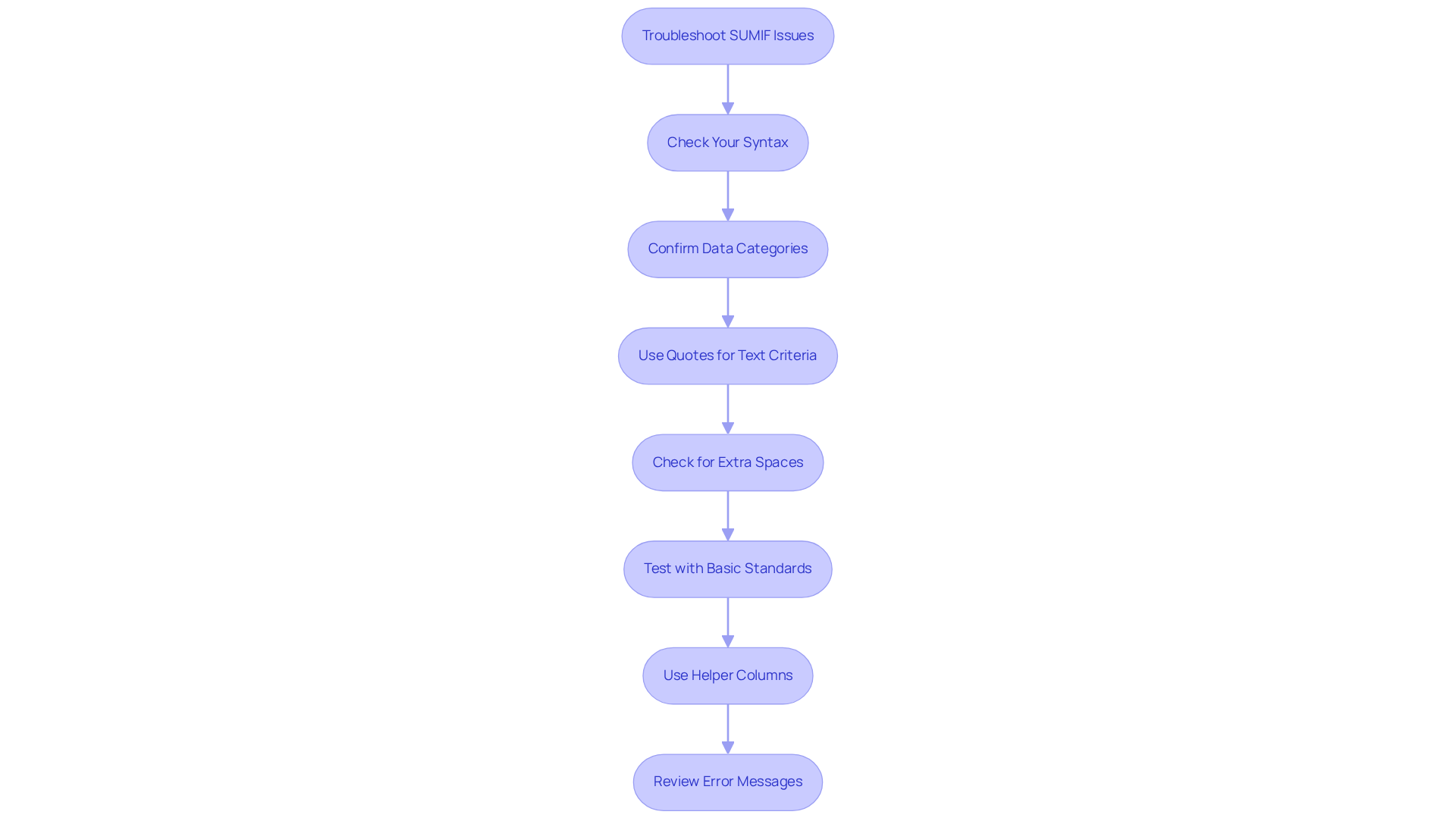
When users learn how to sumif, they often face common issues that can hinder their productivity. Here are some essential troubleshooting tips to help you navigate these challenges:
-
Check Your Syntax: Ensure your formula adheres to the correct syntax. Missing commas or parentheses can lead to frustrating errors.
-
Confirm Data Categories: Make sure the data categories in your selection align with the standard. For instance, if your standard is a number, ensure that the cells in the range are formatted as numbers, not text.
-
Use Quotes for Text Criteria: When using text as a criterion, always enclose it in quotes. For example,
=SUMIF(A1:A10, "Paid", B1:B10). -
Check for Extra Spaces: Extra spaces in your data can cause the SUMIF formula to fail. Utilize the TRIM tool to eliminate any unnecessary spaces.
-
Test with Basic Standards: If your formula isn’t operating as expected, simplify your criteria to see if the formula works with basic conditions. For example, try
=SUMIF(A1:A10, ">0")to check if it sums correctly. -
Use Helper Columns: If you have complex criteria, consider using helper columns to simplify your calculations. This approach can make your formulas easier to manage and troubleshoot.
-
Review Error Messages: Pay attention to any error messages Google Sheets provides. They often offer valuable clues about what might be wrong with your formula.
By following these best practices on how to sumif, you can effectively troubleshoot and resolve issues with the SUMIF function, which will ensure accurate results in your Google Sheets.

Conclusion
Mastering the SUMIF function in Google Sheets is not just a skill; it’s a game changer for anyone serious about data analysis. This powerful tool allows users to sum values based on specific criteria, streamlining financial reporting and data management processes. By simplifying these tasks, the SUMIF function enhances productivity, making it an essential asset in your analytical toolkit.
In this guide, we’ve delved into the key aspects of the SUMIF function - from its definition and syntax to detailed, step-by-step instructions for implementation. We’ve also highlighted common troubleshooting tips and best practices, ensuring you can navigate potential challenges with confidence. Understanding how to effectively use the SUMIF function empowers you to make informed decisions, significantly improving your analytical capabilities.
Embracing the SUMIF function can truly transform your approach to data in Google Sheets. Whether you’re monitoring expenses, evaluating sales data, or compiling financial reports, this function stands as a cornerstone for effective data analysis. As you continue to hone your skills in utilizing SUMIF, you’ll find yourself equipped to make data-driven decisions that can profoundly impact both your professional and personal endeavors.
Frequently Asked Questions
What is the SUMIF function in Google Sheets?
The SUMIF function is a powerful tool used for summing values based on specific conditions in Google Sheets.
What is the syntax of the SUMIF function?
The syntax of the SUMIF function is =SUMIF(range, criterion, [sum_range]).
What does the 'range' parameter in the SUMIF function refer to?
The 'range' parameter refers to the set of cells that are evaluated against the criterion.
What is the 'criterion' in the SUMIF function?
The 'criterion' is the condition that must be met for a cell to be included in the sum. It can be a number, expression, cell reference, or text.
What is the purpose of the 'sum_range' parameter in the SUMIF function?
The 'sum_range' is optional and specifies the exact cells to total. If omitted, Google Sheets sums the cells within the selected range.
Can you provide an example of how to use the SUMIF function?
For example, to sum all sales exceeding $100 in a sales data range, you would write: =SUMIF(A1:A10, ">100").
Why is the SUMIF function beneficial for financial analysis?
The SUMIF function is beneficial for financial analysis as it allows users to quickly aggregate data based on defined criteria, enhancing the ability to analyze financial data and streamline reporting processes.
How have recent enhancements in Google Sheets affected the SUMIF function?
Recent enhancements in Google Sheets have improved the functionality of the SUMIF formula, making it more user-friendly and efficient.

