Master the Google Sheet INDEX Function: A Step-by-Step Guide

Overview

This article serves as a comprehensive guide to mastering the Google Sheets INDEX function. It details the syntax, usage, and common troubleshooting tips associated with this powerful tool. By explaining how to effectively retrieve data from specified ranges, it emphasizes the critical importance of understanding the function's components. Furthermore, it showcases advanced applications, such as combining INDEX with MATCH, to enhance data lookups and improve efficiency.

Introduction

Mastering data retrieval in Google Sheets can fundamentally transform how users engage with their spreadsheets, especially when managing extensive datasets. The INDEX function emerges as an essential tool, facilitating the precise extraction of cell values based on specified row and column numbers.

Nevertheless, many users encounter challenges with its syntax and integration with other functions, such as MATCH, which can significantly enhance efficiency in lookups.

How can one effectively navigate the complexities of the INDEX function to elevate their data management skills and circumvent common pitfalls?

Understand the INDEX Function in Google Sheets

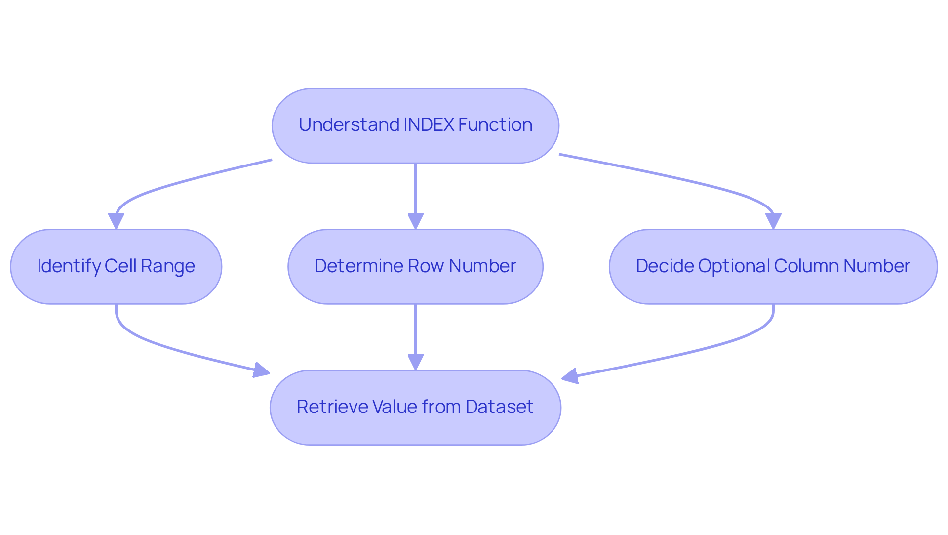
The formula in Google Sheets serves as a powerful tool, enabling users to obtain the value of a cell within a specified range based on its row and column numbers. This functionality is particularly beneficial for extracting information from extensive datasets, where direct cell citations can prove cumbersome. For example, when managing a table of sales data, you can effectively utilize this retrieval method to extract specific sales figures according to their precise location in the table.

The fundamental structure of the formula is INDEX(reference, row, [column]). Here, 'reference' denotes the range of cells, 'row' indicates the row number, and 'column' represents the optional column number. Understanding the google sheet index function is essential for mastering data retrieval in Google Sheets. Data analysts emphasize the significance of the google sheet index function, highlighting that this tool facilitates adaptable and dynamic data retrieval, making it a cornerstone of effective spreadsheet management.

This flowchart shows how to use the INDEX function step-by-step. Start by understanding the function, then follow the arrows to see how to select the range, rows, and columns to get the specific data you need.

Learn the Syntax of the INDEX Function

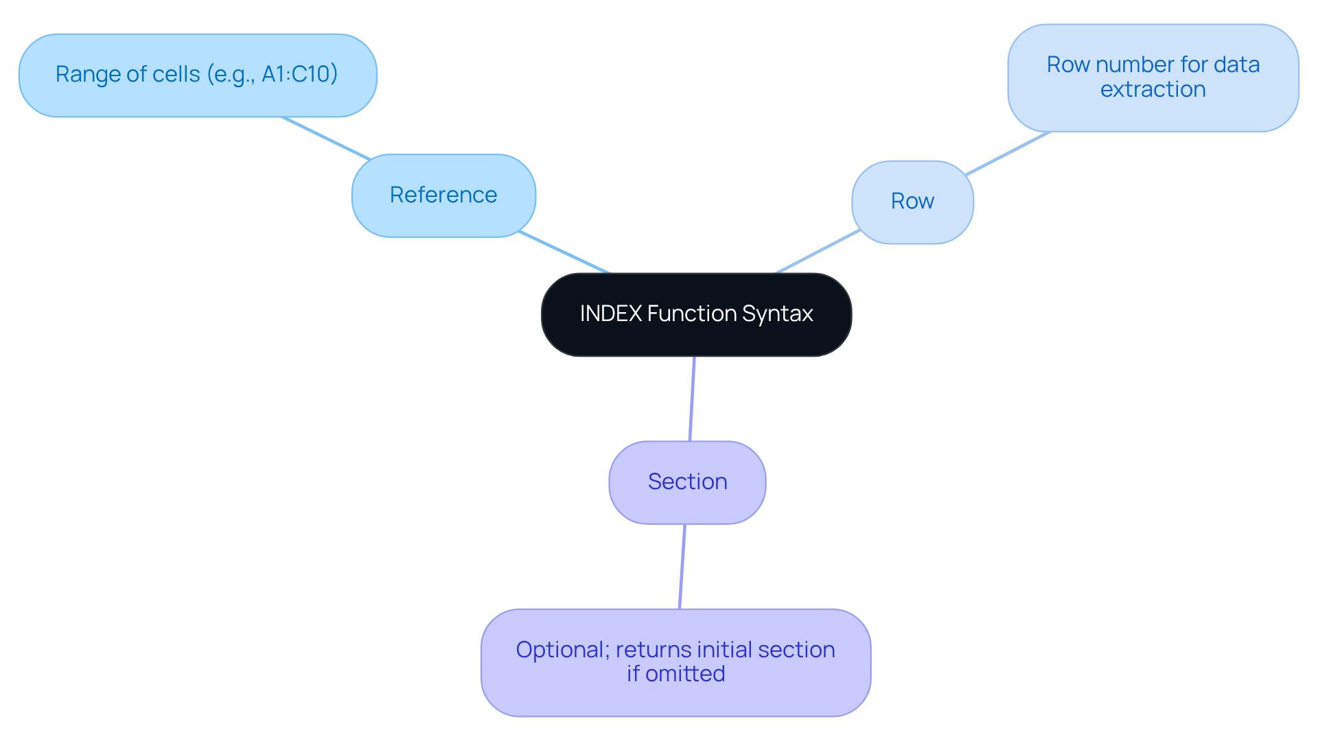
The syntax of the google sheet index function is structured as follows: INDEX(location, row, [column]). Each component serves a distinct purpose:

reference: This denotes the range of cells from which data will be retrieved, such as A1:C10.
row: This indicates the row number within the source from which to extract a value. If excluded, this parameter defaults to 0, returning the entire set specified.
section: This optional parameter specifies the section number in the reference. If omitted, the function defaults to returning the initial section specified.

For example, the formula =INDEX(A1:C10, 2, 3) retrieves the value located in the second row and third column of the defined range. Mastering the google sheet index function syntax is essential for effectively utilizing the data retrieval tool across various applications, especially in finance where accurate data retrieval is critical.

Experts emphasize that understanding the elements of this formula can significantly enhance data management skills. As one specialist noted, "The array tool provides greater flexibility and capability for handling intricate data," which is especially beneficial for finance professionals aiming to optimize their workflows. However, caution is advised; specifying offsets outside the defined input range can lead to errors.

The center shows the main function, and the branches provide details on each part. Follow the branches to learn about the reference range, row number, and optional section—each is vital for using the function correctly.

Combine INDEX with MATCH for Advanced Lookups

To enhance the capabilities of the lookup tool, consider integrating it with the MATCH operation. The MATCH operation identifies the location of a specified value within a defined range, which can subsequently serve as an argument in the ARRAY formula. The syntax for merging these functions is as follows:

=INDEX(reference, MATCH(lookup_value, lookup_range, [match_type]))

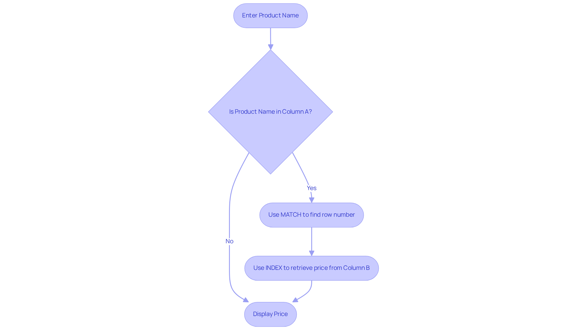
For instance, if you have a catalog of products in column A and their corresponding prices in column B, and you seek to determine the price of a particular product, you can apply:

=INDEX(B:B, MATCH("Product Name", A:A, 0))

In this formula, MATCH identifies the row number of "Product Name" in column A, while INDEX retrieves the associated price from column B. This powerful combination facilitates more versatile lookups, particularly when managing extensive datasets.

This flowchart guides you through using INDEX and MATCH. Start by entering the product name, check if it's in the catalog, find its row, retrieve the price, and then display the result.

Troubleshoot Common Issues with the INDEX Function

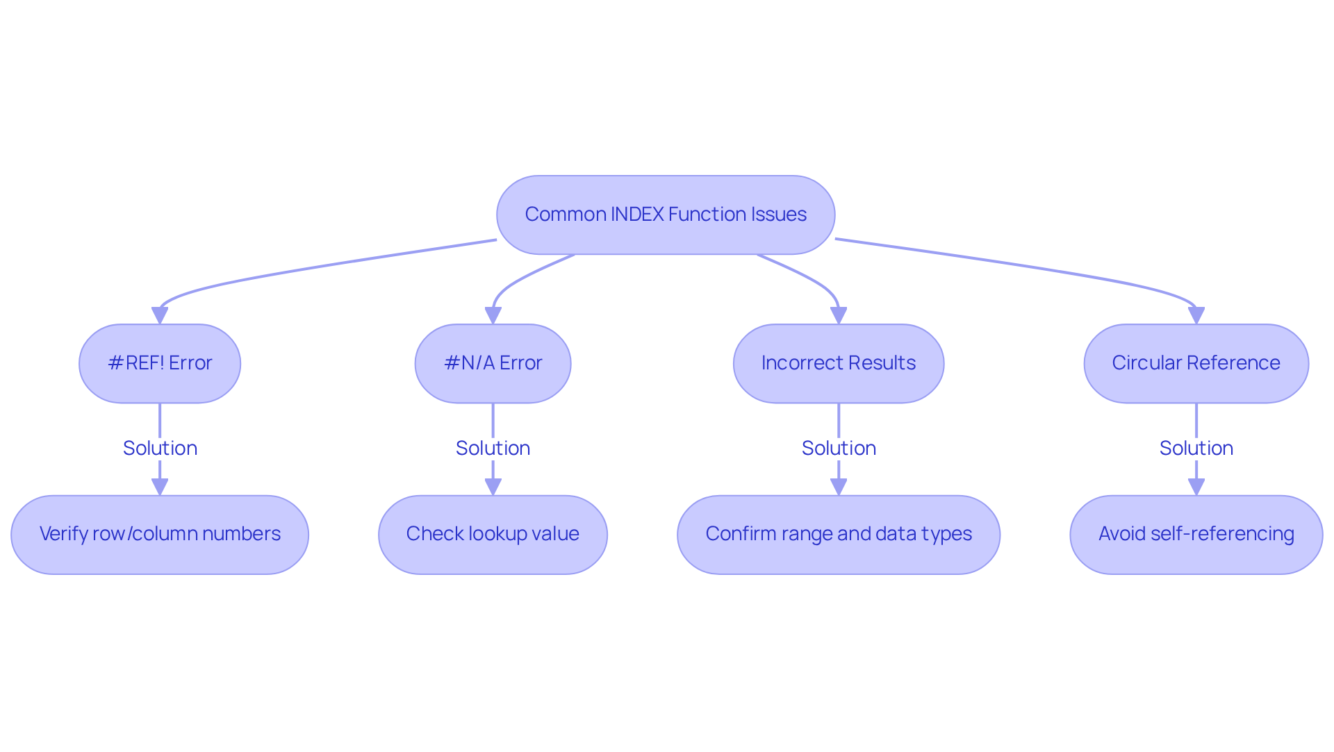
When utilizing the Google Sheet INDEX function, users may encounter several common issues that can disrupt their workflow. Here are some essential troubleshooting tips to address these challenges:

#REF! Error: This error arises when the specified row or column number falls outside the reference range. It is crucial to verify that your row and column numbers remain within the defined bounds of the specified range.
#N/A Error: This indicates that the MATCH function was unable to locate the lookup value. To resolve this, double-check the lookup value to ensure its presence within the lookup range.
Incorrect Results: If the results appear inaccurate, it is important to confirm that both the range and the row/column numbers are correctly indicated. Additionally, ensure that the data types align (e.g., text versus numbers).
Circular Reference: This issue occurs when the formula references its own cell. To avoid creating circular references, ensure that your formula does not point back to its own cell.

By understanding these common issues and their respective solutions, users can troubleshoot effectively, including the Google Sheet INDEX function, to maintain a seamless workflow without unnecessary interruptions.

Follow the arrows to see common issues with the INDEX function. Each box represents a specific error and its solution — address the issue by following the flow to the right fix.

Conclusion

Mastering the Google Sheets INDEX function is essential for unlocking a powerful tool that facilitates efficient data retrieval and management. By grasping its syntax and functionality, users can streamline their workflows, making it significantly easier to extract specific information from extensive datasets. This function not only boosts productivity but also serves as a foundational element for more complex operations, such as its integration with the MATCH function for advanced lookups.

Key points throughout this article emphasize the basic structure of the INDEX function, its syntax, and practical examples of effective application. Furthermore, the exploration of the INDEX and MATCH combination illustrates how this synergy allows for dynamic and versatile data lookups. Common issues and troubleshooting tips are also addressed, empowering users to navigate potential challenges with confidence.

The significance of the INDEX function in Google Sheets is profound. It empowers users to manage data efficiently, minimize errors, and enhance analytical capabilities. Embracing this tool leads to better data-driven decisions and improved productivity. For anyone seeking to optimize their use of Google Sheets, mastering the INDEX function is a crucial step toward achieving greater efficiency and accuracy in data management.

Frequently Asked Questions

What is the INDEX function in Google Sheets?

The INDEX function in Google Sheets is a formula that allows users to obtain the value of a cell within a specified range based on its row and column numbers.

How does the INDEX function benefit users?

The INDEX function is particularly beneficial for extracting information from extensive datasets, making it easier to retrieve specific values without cumbersome direct cell citations.

What is the basic structure of the INDEX formula?

The basic structure of the INDEX formula is INDEX(reference, row, [column]), where 'reference' is the range of cells, 'row' is the row number, and 'column' is the optional column number.

Why is understanding the INDEX function important?

Understanding the INDEX function is essential for mastering data retrieval in Google Sheets, as it facilitates adaptable and dynamic data extraction, which is crucial for effective spreadsheet management.

Who emphasizes the importance of the INDEX function?

Data analysts emphasize the significance of the INDEX function for its role in facilitating effective and dynamic data retrieval in spreadsheets.