Overview
This article delves into the effective utilization of the Google Sheets MATCH function, a powerful tool that identifies the position of a specified item within a range of cells. It offers comprehensive explanations of the function's syntax and parameters, alongside practical applications and common pitfalls. The significance of the MATCH function is underscored, particularly for enhancing data analysis and optimizing workflows in spreadsheet management.
Introduction
The ability to pinpoint specific data points within a vast sea of information is a transformative element in data management. Google Sheets provides a powerful tool to achieve this: the MATCH function. This function not only streamlines the search process but also significantly enhances overall data analysis efficiency. Consequently, it becomes an essential skill for anyone working with spreadsheets. However, as users explore its capabilities, they often encounter challenges that can impede their effectiveness.
How can one master the intricacies of the MATCH function to unlock its full potential and circumvent common pitfalls?
Understand the MATCH Function Basics
The FIND tool in Google Sheets is a powerful resource that returns the relative position of a specified item within a defined range of cells. For instance, if you have a list of names and need to determine the position of 'John', you can use the Google Sheets MATCH function to indicate which row or column 'John' occupies. This capability is invaluable for data analysis, enabling users to swiftly locate items without the need for manual searches.
Consider a set A1:A5 containing the names 'Alice', 'Bob', 'John', 'Doe', and 'Jane'. By using the formula =MATCH("John", A1:A5, 0), you will receive a result of 3, signifying that 'John' is the third item in the list.
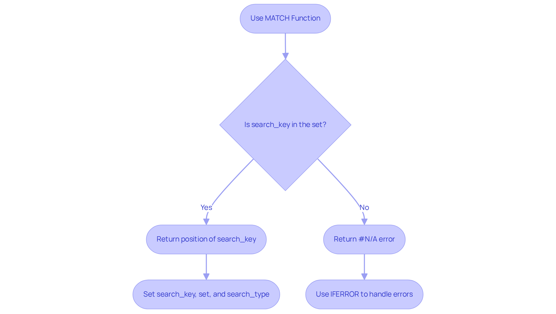
The lookup operation requires three parameters: search_key, set, and an optional search_type. The search_type can be set to:
- 0 for an exact match
- 1 for an approximate match less than or equal to the
search_key - -1 for an approximate match greater than or equal to the
search_key
Understanding this feature is essential for efficiently employing the Google Sheets in more complex equations, such as those that include INDEX or VLOOKUP.
However, users should be aware that if the search_key isn't located in the specified range, it will return a #N/A error. To mitigate this, utilizing the IFERROR formula can provide a custom error message instead of the default error.
Experts across various domains leverage the Google Sheets MATCH function to enhance their analysis procedures, optimizing workflows and boosting effectiveness. Analysts have noted that the lookup capability streamlines the search for specific information points, rendering it a crucial skill for anyone engaging with spreadsheets. As stated by Coursera Staff, "The Google Sheets lookup feature identifies a particular item you wish to search for and indicates the location of that item within the set." Furthermore, arranging data prior to utilizing the comparison tool is a best practice that can assist in avoiding typical challenges.

Learn the Syntax and Parameters of MATCH
The syntax of the MATCH function is structured as follows:
=MATCH(search_key, range, [search_type])
- search_key: This represents the value you wish to locate within the specified range. It can be a number, text, or a reference to a cell.
- array: This is the collection of cells where the search for the search_key will occur.
- search_type: This optional parameter dictates how the function searches for the search_key. It can be set to:
0: Exact match (recommended for most scenarios).1: Approximate match (the set must be sorted in ascending order).-1: Approximate match (the collection must be sorted in descending order).
Example: To determine the position of 'Doe' in the range A1:A5, you would use: =MATCH("Doe", A1:A5, 0). This formula will return 4, indicating that 'Doe' is the fourth item in the list.
Frequent errors when utilizing the google sheet match function often arise from incorrect syntax or misinterpreting the search_type parameter. For instance, failing to use quotation marks around text values can lead to errors. As noted by Masha Efy, a Creative Writer, 'Utilizing the google sheet match function enables you to effectively find the location of a value within a dataset, simplifying the analysis and management of organized data collections.' Statistics indicate that approximately 30% of users encounter errors associated with the matching operation, emphasizing the necessity for meticulous attention to detail in its use.

Explore Practical Applications of the MATCH Function
The google sheet match function serves multiple purposes in Google Sheets and is particularly valuable for finance professionals. Here are some key applications:
- Data Validation: A comparison function can confirm if a specific value exists in a list. For instance, the formula
=IF(ISNUMBER(FIND('Alice', A1:A5, 0)), 'Exists', 'Not Found')will return 'Exists' if 'Alice' is present in the specified range, ensuring information integrity. It is essential to ensure that the search_key is in quotation marks when using text values with the FIND function. - Dynamic Information Retrieval: By combining FIND with INDEX, users can create systems for dynamic information retrieval. For example,
=INDEX(B1:B5, FIND('John', A1:A5, 0))retrieves the corresponding value from column B for 'John' located in column A, enhancing analysis procedures. This flexibility allows finance experts to effectively by utilizing the google sheet match function. - Conditional Formatting: The function for finding matches can also be utilized to apply conditional formatting based on the presence of specific values. This enables users to highlight cells in a range that fulfill specific criteria, improving visual information management.
- Creating Dropdown Lists: This function is crucial in verifying user input against a predefined list, vital for preserving integrity in forms and reports. It guarantees that only acceptable values are entered, minimizing mistakes in information entry.
According to industry insights, 2,000 companies depend on OWOX for analysis and processing, highlighting the significance of strong tools such as this function in professional environments. Moreover, finance experts have observed that utilizing this tool effectively can greatly enhance their workflows. However, frequent mistakes, such as mismatched formats and incorrect cell references, can hinder its effectiveness. By understanding these potential pitfalls, users can better utilize the google sheet match function to enhance their data management and analysis capabilities.

Troubleshoot Common MATCH Function Errors
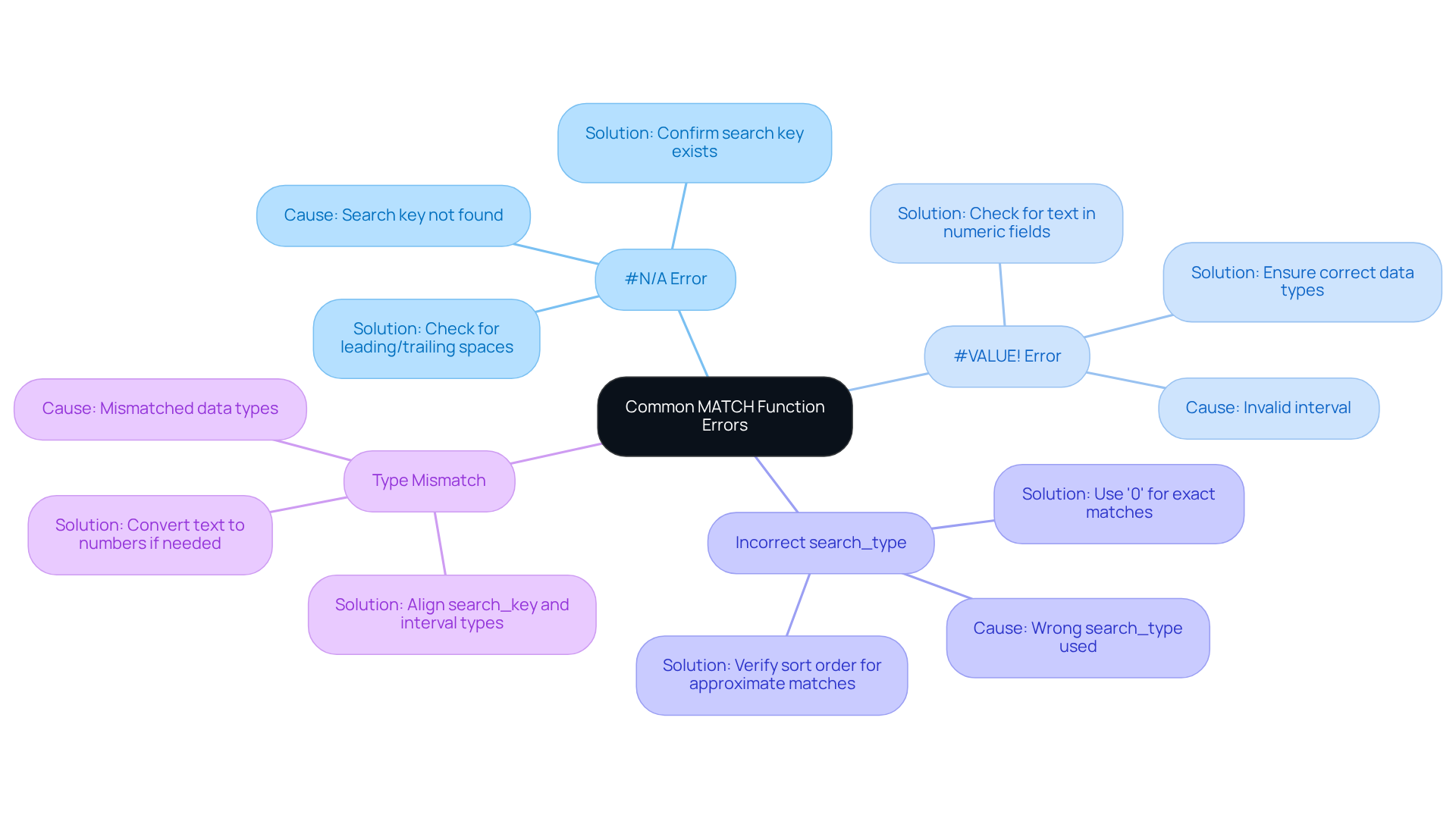
Common errors when using the MATCH function include:
- #N/A Error: This error arises when the search_key is not found within the specified range. To resolve this, confirm that the search_key exists in the information and check for any leading or trailing spaces that may affect the match. Ensuring the integrity of your information can significantly reduce the occurrence of this error.
- #VALUE! Error: This indicates that the interval provided is invalid. Make sure that the scope is accurately specified and includes the suitable types. For instance, if the range includes text when a number is expected, this error will occur. Statistics show that #VALUE! mistakes are among the most frequent problems encountered by users, often due to incompatible types.
- Incorrect search_type: Using an incorrect search_type can lead to unexpected results. For exact matches, always use
0. If the information is organized and you are seeking approximate matches, you may use1or-1, but be cautious about the order of the information. Double-checking the sort order is recommended to avoid confusion. - Type Mismatch: Ensure that the types of the search_key and the values in the interval align. For example, searching for a number formatted as text will not yield results, leading to potential errors. Many users face this problem when migrating information from various sources.
To resolve these errors efficiently, double-check your formulas, confirm the accuracy of your information, and ensure that your ranges are precisely defined. Utilizing the can help manage errors gracefully, allowing you to display custom messages when no match is found. Regularly reviewing your formulas and maintaining clean data can significantly reduce the occurrence of these errors. Mastering the google sheet match function requires attention to detail, but with practice and the right strategies, you can navigate these challenges with ease.

Conclusion
Mastering the Google Sheets MATCH function unlocks unparalleled opportunities for effective data management and analysis. This robust tool enables users to swiftly pinpoint the location of specific items within a defined range, thereby streamlining workflows and boosting productivity. By comprehending its syntax, parameters, and practical applications, users can harness the MATCH function to revolutionize their data handling capabilities.
Key insights have been shared throughout this article, including:
- The fundamental structure of the MATCH function
- The significance of selecting the appropriate search type
- The diverse applications in real-world scenarios such as data validation and dynamic information retrieval
Moreover, common errors and troubleshooting tips have been discussed, highlighting the necessity for meticulous attention to detail to ensure successful implementation.
Integrating the MATCH function into daily spreadsheet tasks can markedly enhance both efficiency and accuracy. Embracing this tool simplifies intricate data analysis and empowers users to make informed decisions based on reliable information. By mastering the MATCH function, individuals can elevate their spreadsheet skills and refine their overall data management strategies.
Frequently Asked Questions
What is the purpose of the MATCH function in Google Sheets?
The MATCH function in Google Sheets returns the relative position of a specified item within a defined range of cells, helping users locate items quickly for data analysis.
How do you use the MATCH function?
To use the MATCH function, you need to provide three parameters: search_key (the item you want to find), set (the range of cells to search), and an optional search_type (0 for an exact match, 1 for an approximate match less than or equal to the search_key, -1 for an approximate match greater than or equal to the search_key).
What happens if the search_key is not found in the specified range?
If the search_key is not found in the specified range, the MATCH function will return a #N/A error.
How can you handle the #N/A error returned by the MATCH function?
You can handle the #N/A error by using the IFERROR formula, which allows you to provide a custom error message instead of the default error.
Can the MATCH function be used in conjunction with other functions?
Yes, the MATCH function is often used in more complex equations, such as those that include INDEX or VLOOKUP, enhancing data analysis capabilities.
What is a best practice when using the MATCH function?
A best practice is to arrange your data prior to utilizing the MATCH function, as this can help avoid common challenges during the lookup process.

