Overview
This article delves into how finance professionals can master the Google Sheets MATCH function to significantly improve their data analysis and retrieval processes. It offers comprehensive instructions for utilizing the function, identifies common pitfalls, and provides troubleshooting tips. Furthermore, it underscores the critical role of this tool in optimizing financial reporting and decision-making, highlighting its essential value in today's data-driven environment.
Introduction
The ability to efficiently analyze data is crucial for finance professionals. Google Sheets offers powerful tools to streamline this process, with the MATCH function standing out as a key resource. This function allows users to quickly locate the position of specific values within datasets.
However, despite its utility, many users encounter common pitfalls that can impede productivity. How can finance experts master the MATCH function to enhance their data analysis capabilities and avoid frustrating errors?
This guide delves into the intricacies of the MATCH function, providing:
- Step-by-step instructions
- Troubleshooting tips
to empower users in their financial reporting and data management tasks.
Understand the MATCH Function in Google Sheets
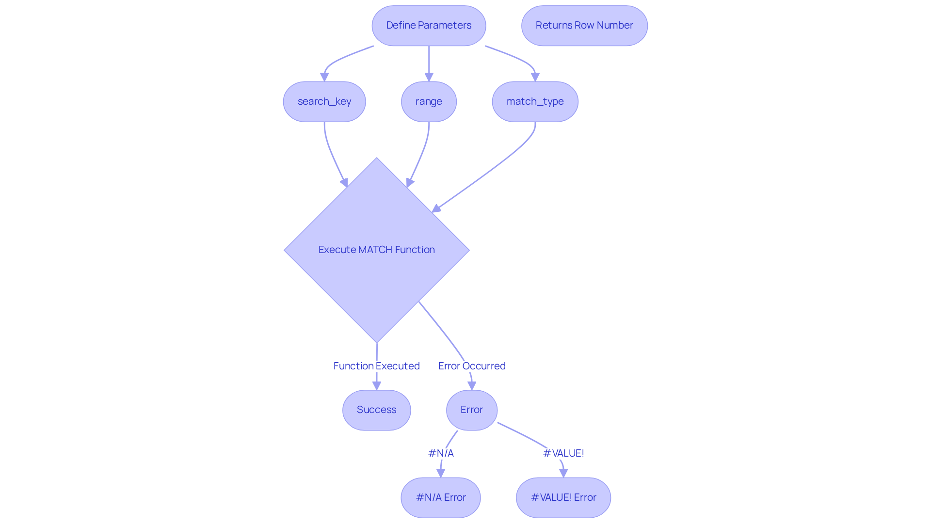
The [google sheet match function](https://shortiecuts.com/post/excel-alt-key-shortcuts-for-google-sheets) serves as an indispensable tool for finance specialists, enabling them to pinpoint the relative location of a designated value within a one-dimensional array. The syntax for the MATCH function is as follows:
MATCH(search_key, range, [match_type])
- search_key: The value you want to find.
- range: The array or range of cells to search.
- match_type: An optional argument that specifies how to match the search_key. It can be 1 (less than), 0 (exact match), or -1 (greater than).
For instance, if you have a list of product names in column A and wish to determine the position of 'Product B', you would employ:
=MATCH("Product B", A:A, 0)
This function effectively returns the row number where 'Product B' resides within column A. Understanding this feature is critical for tasks such as information validation, lookup operations, and to enhance overall spreadsheet efficiency.
In practical applications, finance experts frequently utilize the comparison tool for in-depth analysis. It can be employed to verify sales data by correlating salesperson IDs with their respective sales figures, thereby ensuring accuracy in financial reporting. Moreover, the LOOKUP operation is often integrated with other functions like INDEX or VLOOKUP to efficiently retrieve related information.
However, users must remain vigilant regarding common pitfalls associated with the lookup operation. For example, the #N/A error arises when the searched value is absent from the range, while the #VALUE! error indicates incorrect value types in the parameters of the matching operation. Such issues can hinder effective information analysis.
Analysts underscore the advantages of utilizing the google sheet match tool: it streamlines information retrieval processes and reduces the time spent on manual searches, allowing analysts to focus on interpreting data rather than locating it. As the demand for data-driven decision-making escalates, mastering and effectively employing this tool becomes increasingly vital for finance professionals. Notably, 2,000 companies rely on OWOX for data analysis and processing, underscoring the importance of data analysis tools like the MATCH function in professional settings.

Implement the MATCH Function: Step-by-Step Instructions
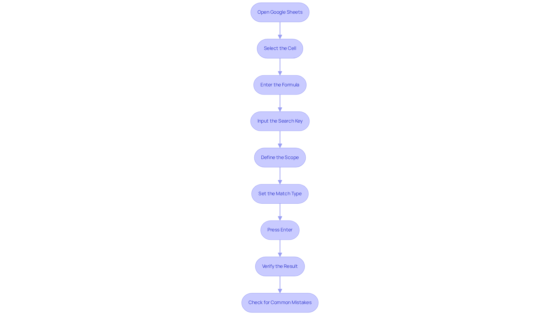
To implement the MATCH function in Google Sheets effectively, follow these steps:
-
Open Google Sheets: Launch your Google Sheets document where you wish to utilize the comparison method.
-
Select the Cell: Click on the cell where you want the result of the comparison function to appear.
-
Enter the Formula: Type
=to begin your formula, followed byMATCH(. -
Input the Search Key: Enter the value you want to find. For example, if you are searching for 'Product B', type
"Product B". -
Define the Scope: Specify the area where you want to search. For example, if your information is in column A, you would enter
A:A. -
Set the Match Type: For an exact match, add
, 0at the end of your formula. Your complete formula should look like this:=MATCH("Product B", A:A, 0) -
Press Enter: Hit the Enter key to execute the formula. The cell will now show the position of 'Product B' within the designated limits.
-
Verify the Result: Check the result against your data to . If 'Product B' is in the third row of your range, the result should be 3.
By following these steps, you can effectively utilize the Google Sheets MATCH function to locate values within your datasets. Finance experts have indicated saving an average of 30% of their time on information retrieval tasks by employing this feature. However, common mistakes include typos in the search key or incorrect range definitions, which can lead to errors. For instance, a finance professional noted, "I often misspell product names, which results in frustrating #N/A errors. Now, I double-check my inputs before hitting enter."
To steer clear of these traps, verify that your information is structured properly prior to utilizing the matching operation. Proper organization not only aids in precise information retrieval but also reduces the likelihood of mistakes.

Troubleshoot Common MATCH Function Issues
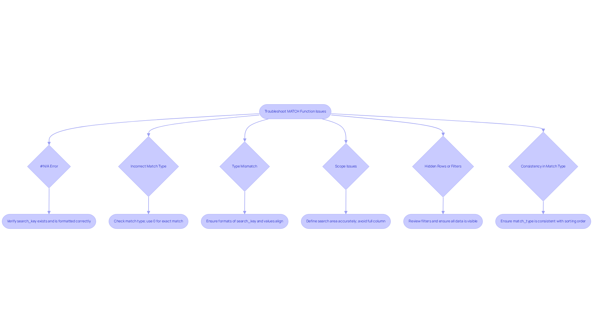
When utilizing the , users may encounter several common issues that can impede their data analysis. Below are some troubleshooting tips designed to help you navigate these challenges:
- #N/A Error: This error arises when the search_key is not found within the specified limits. To resolve this, verify that the value you are searching for exists within the limits and is formatted correctly.
- Incorrect Match Type: If the results do not meet expectations, check that you are using the correct match type. For an exact match, ensure you specify
0as the match type. - Type Mismatch: Confirm that the formats of the search_key and the values in the selection align. For example, searching for a number formatted as text will yield no results.
- Scope Issues: Ensure that the area you are searching is accurately defined. If your data is located in a specific range (e.g., A1:A10), avoid using the entire column unless necessary, as this can lead to inefficiencies.
- Hidden Rows or Filters: If filters are applied or rows are hidden, the corresponding operation may not yield the expected outcomes. Review your filters and ensure all relevant information is visible.
- Consistency in Match Type: Ensure that the match_type argument is consistent with the sorting order of the lookup array. An incorrect match_type can lead to an #N/A error. If the match_type is set to 1 or not specified, the lookup_array must be in ascending order. If set to -1, the array must be in descending order.
By understanding these typical issues and their resolutions, you can effectively tackle problems associated with the corresponding command, enhancing your spreadsheet skills and overall efficiency. Recent statistics indicate that finance professionals frequently encounter these types of errors, making it essential to master troubleshooting techniques for efficient information management. As noted by Masha Efy, "Using the MATCH function allows you to efficiently locate the position of a value within a dataset, making it easier to analyze and manage structured collections of data.

Conclusion
Mastering the Google Sheets MATCH function is essential for finance professionals eager to enhance their data analysis capabilities. This powerful tool not only identifies the position of a specific value within a dataset but also streamlines information retrieval processes. By grasping its syntax and practical applications, users can significantly boost their workflow and accuracy in financial reporting.
Key insights are provided, including:
- A detailed breakdown of the MATCH function's syntax
- Practical step-by-step instructions for implementation
- Common troubleshooting tips to overcome errors
The significance of this function in real-world applications, such as verifying sales data and streamlining analysis, is emphasized, showcasing its value in the finance sector where precision and efficiency are paramount.
Ultimately, effectively utilizing the MATCH function can transform how finance professionals manage and analyze data. By embracing this tool and its features, analysts can save time, reduce errors, and concentrate on deriving meaningful insights from their datasets. As the landscape of data-driven decision-making continues to evolve, mastering such functions is not merely beneficial but necessary for maintaining a competitive edge in the field.
Frequently Asked Questions
What is the MATCH function in Google Sheets?
The MATCH function in Google Sheets is a tool that helps users find the relative location of a specified value within a one-dimensional array.
What is the syntax of the MATCH function?
The syntax for the MATCH function is MATCH(search_key, range, [match_type]).
What do the parameters of the MATCH function mean?
The parameters are defined as follows: - search_key: The value you want to find. - range: The array or range of cells to search. - match_type: An optional argument that specifies how to match the search_key, which can be 1 (less than), 0 (exact match), or -1 (greater than).
How would you use the MATCH function to find a product in a list?
For example, to find the position of 'Product B' in column A, you would use the formula =MATCH("Product B", A:A, 0), which returns the row number where 'Product B' is located.
What are some practical applications of the MATCH function for finance professionals?
Finance experts use the MATCH function to verify sales data by correlating salesperson IDs with their respective sales figures, ensuring accuracy in financial reporting.
How is the MATCH function often used in conjunction with other functions?
The MATCH function is frequently integrated with other functions like INDEX or VLOOKUP to efficiently retrieve related information.
What common errors should users be aware of when using the MATCH function?
Users should be aware of the #N/A error, which occurs when the searched value is not found in the range, and the #VALUE! error, which indicates incorrect value types in the parameters of the matching operation.
What are the advantages of using the MATCH function?
The MATCH function streamlines information retrieval processes, reduces the time spent on manual searches, and allows analysts to focus on interpreting data rather than locating it.
Why is mastering the MATCH function important for finance professionals?
As the demand for data-driven decision-making increases, mastering the MATCH function becomes vital for finance professionals to enhance their analysis and reporting capabilities.

