Master VLOOKUP Across Multiple Sheets for Financial Success

Introduction

Mastering the VLOOKUP function can revolutionize how financial professionals manage data across multiple sheets. It streamlines analysis and enhances accuracy, making it an indispensable tool in your arsenal. This guide explores the intricacies of VLOOKUP, providing essential techniques and troubleshooting tips that empower users to fully leverage its capabilities.

However, as users navigate the complexities of this powerful tool, they often face challenges that can hinder their progress. How can one effectively overcome these hurdles to ensure seamless data retrieval and reporting? By understanding the common pitfalls and employing strategic solutions, you can transform your data handling processes and achieve greater efficiency in your reporting.

Understand VLOOKUP Syntax and Basics

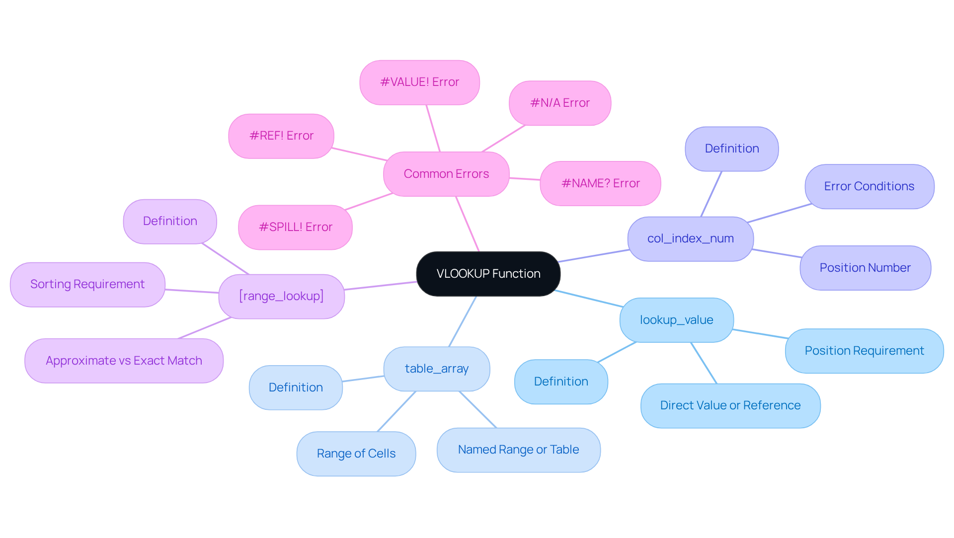
To effectively harness the power of the VLOOKUP function, it's crucial to understand its syntax and key components. The basic syntax is as follows:

=VLOOKUP(lookup_value, table_array, col_index_num, [range_lookup])

lookup_value: This is the value you want to search for in the first column of your specified table. It’s essential that this value is positioned in the first section of the range for VLOOKUP to function correctly.
table_array: This refers to the range of cells containing the data you wish to retrieve.
col_index_num: This indicates the position number in the table from which to extract the information, with the first position designated as 1. Be aware that if col_index_num is less than 1, a #VALUE! error will occur.
[range_lookup]: This optional argument can be set to TRUE for an approximate match or FALSE for an exact match. If range_lookup is TRUE, the first section must be sorted to avoid unexpected results.

Example:
To find the price of a product based on its ID, your formula might look like this:

=VLOOKUP(A2, B2:D10, 3, FALSE)

This formula searches for the value in cell A2 within the first column of the range B2:D10 and returns the corresponding value from the third column of that range. Understanding this syntax is crucial for applying VLOOKUP multiple sheets effectively.

Common Errors:
Be mindful that if the lookup_value is smaller than the smallest value in the first column of the table_array, a #N/A error will occur when range_lookup is TRUE. Additionally, if col_index_num exceeds the number of columns in the table_array, a #REF! error will be generated. Familiarity with these potential obstacles will enhance your ability to troubleshoot and optimize your applications. Furthermore, remember that wildcard characters can be utilized in the lookup function when range_lookup is FALSE, and using absolute references allows you to fill down a formula while maintaining the same lookup range.

The center represents the VLOOKUP function, and each branch shows a key component. Follow the branches to learn about each part's role and how they work together.

Apply VLOOKUP Across Multiple Sheets

To effectively apply VLOOKUP across multiple sheets, follow these steps:

Identify the Sheets: Determine which sheets contain the data you need to reference. For example, consider two sheets: 'SalesData' and 'ProductInfo'.
Construct the VLOOKUP Formula: Use the following syntax to reference another sheet:

=VLOOKUP(lookup_value, 'SheetName'!table_array, col_index_num, [range_lookup])

For instance, to look up a product ID from 'SalesData' in 'ProductInfo', your formula looks like this:

=VLOOKUP(A2, 'ProductInfo'!A2:C10, 2, FALSE)

Drag the Formula: After entering the formula in the desired cell, drag the fill handle down to apply it to other cells in the vertical section. This ensures a consistent application across your dataset.
Check for Errors: Verify that the lookup values exist in the referenced sheet to avoid errors such as #N/A, which can disrupt your analysis.

Example: If you have product IDs in column A of 'SalesData' and want to retrieve product names from 'ProductInfo', your formula dynamically pulls the names based on the IDs. This enhances the efficiency of your data analysis process. This method is particularly beneficial for finance professionals, as it allows for streamlined reporting and accurate data retrieval through VLOOKUP across multiple sheets and datasets.

Follow the arrows from one step to the next to learn how to use VLOOKUP effectively. Each box shows what you need to do at that stage, helping you avoid mistakes and streamline your data analysis.

Troubleshoot Common VLOOKUP Issues

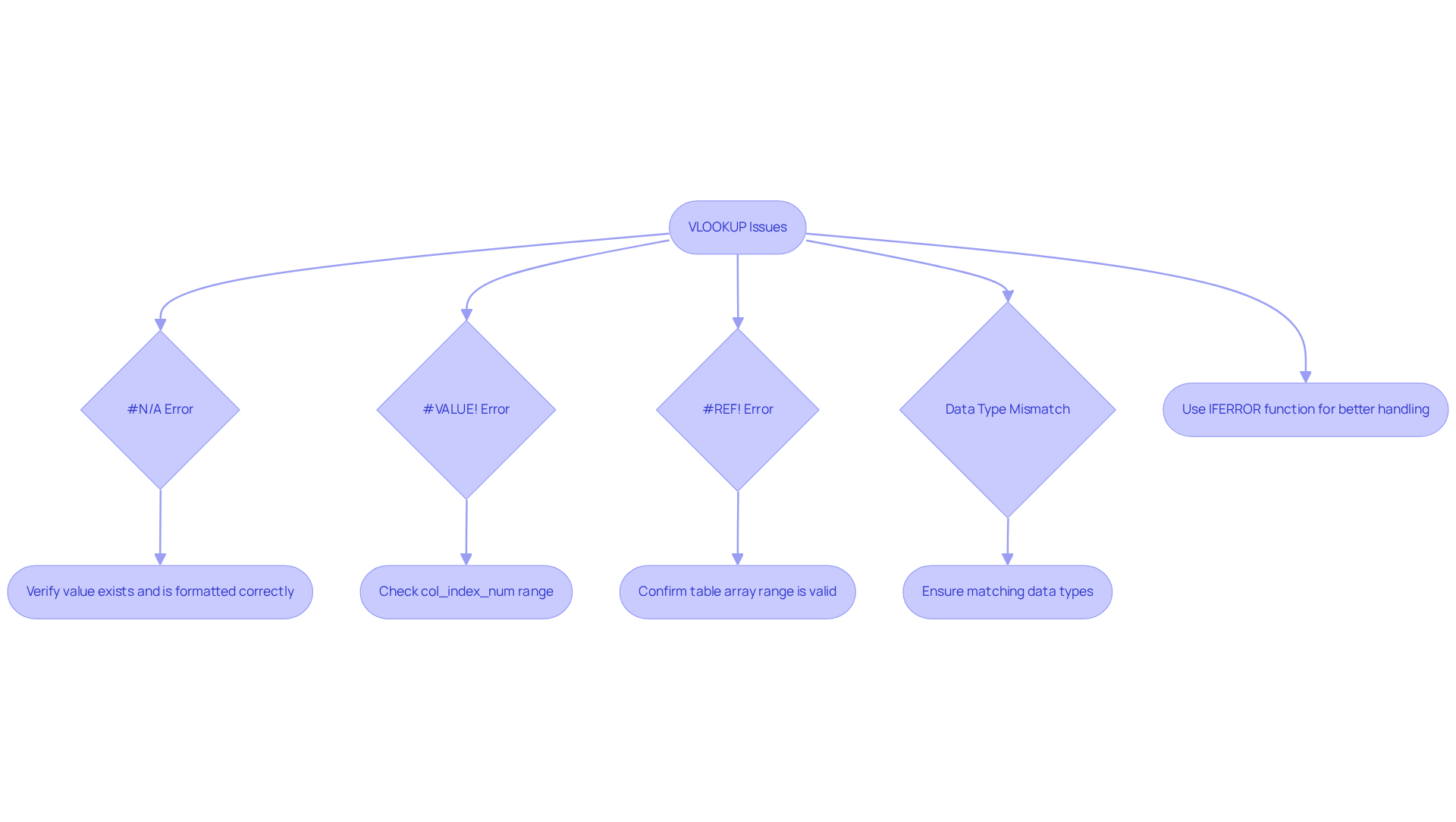
When using VLOOKUP, several common issues may arise. Here’s how to troubleshoot them effectively:

#N/A Error: This error occurs when the lookup item is not present in the first column of the table array. To resolve this, verify that the value exists and is formatted correctly. Approximately 20% of users encounter this error due to mismatched data types or formatting inconsistencies.
#VALUE! Error: This error signifies that the col_index_num is either less than 1 or exceeds the total number of fields in the table array. Ensure that your index is within the correct range.
#REF! Error: This error indicates that the specified table array is invalid. Confirm that the range you have defined exists and is accurate.
Data Type Mismatch: Ensure that the data types of the lookup item and the first column of the table array match. For instance, both should be formatted as text or numbers to avoid errors.

If you encounter a #N/A error, check if the lookup value in your formula corresponds to the value in the referenced sheet. To manage errors more effectively, consider using the IFERROR function:

=IFERROR(VLOOKUP(A2, 'ProductInfo'!A2:C10, 2, FALSE), "Not Found")

This formula will display 'Not Found' instead of an error message, enhancing the user experience and maintaining workflow efficiency. By addressing these common issues, you can streamline your financial modeling processes and improve data accuracy.

Follow the arrows to identify and resolve common VLOOKUP errors. Each path leads you through specific troubleshooting steps for that error type, helping you fix issues efficiently.

Explore Advanced VLOOKUP Techniques

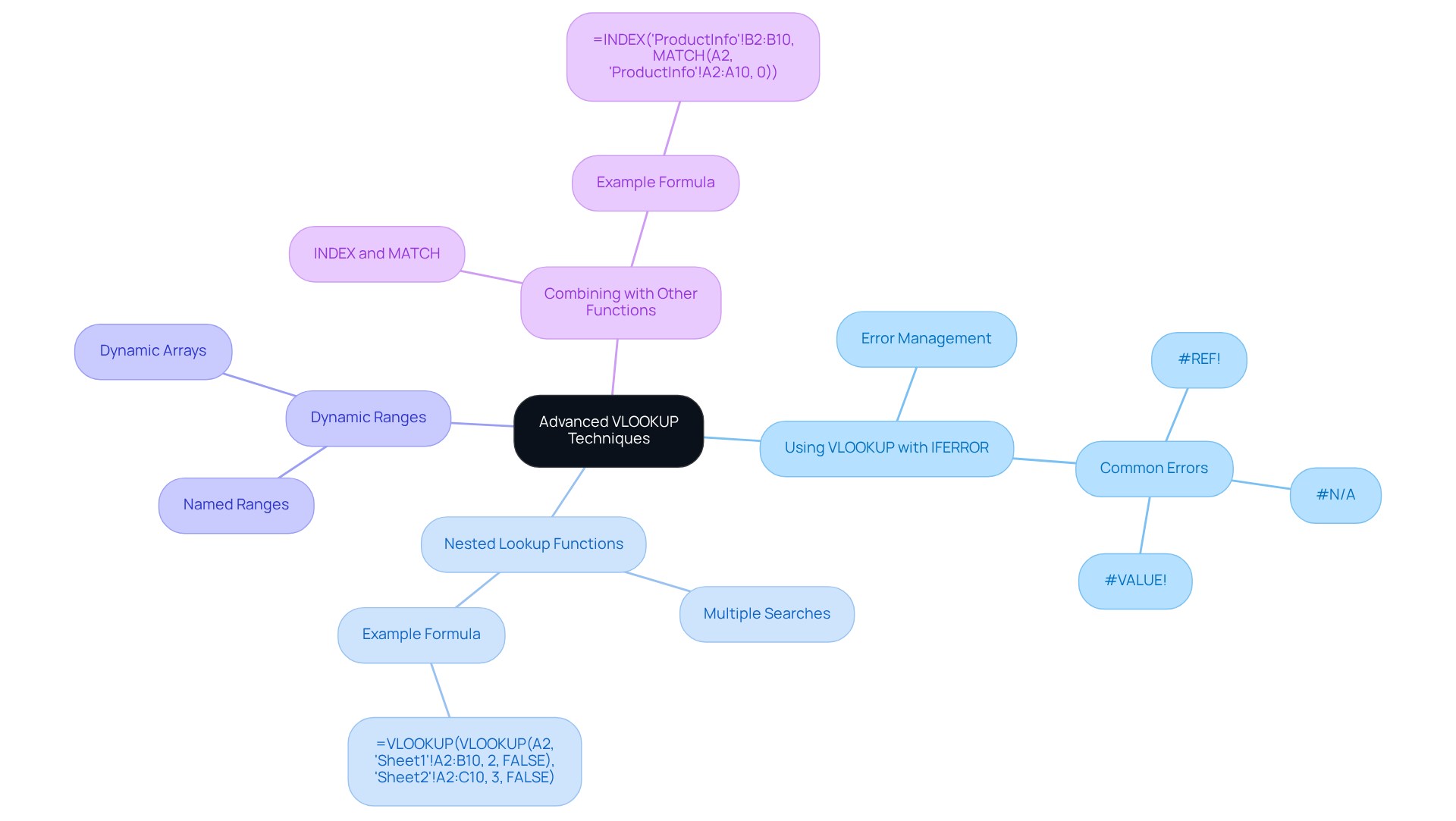
To elevate your VLOOKUP skills, consider these advanced techniques:

Using VLOOKUP with IFERROR: Combining VLOOKUP with IFERROR effectively manages errors, ensuring a cleaner output. This method is particularly beneficial in financial analysis, where information integrity is crucial. Watch out for common mistakes like #REF!, #N/A, and #VALUE!, as these can disrupt your information retrieval process.
Nested Lookup Functions: Nesting lookup functions allows for multiple searches within a single formula. For example:

=VLOOKUP(VLOOKUP(A2, 'Sheet1'!A2:B10, 2, FALSE), 'Sheet2'!A2:C10, 3, FALSE)

This retrieves data from two different sheets based on a lookup value, streamlining complex data retrieval processes. Notably, a significant percentage of finance professionals utilize nested VLOOKUPs for intricate lookups in financial modeling and reporting.

Dynamic Ranges: Implementing named ranges or dynamic arrays enhances the flexibility of your lookup formulas. This adaptability is essential for efficiently managing large datasets.
Combining with Other Functions: Pairing the lookup function with tools like INDEX and MATCH can yield more complex lookups. For instance:

=INDEX('ProductInfo'!B2:B10, MATCH(A2, 'ProductInfo'!A2:A10, 0))

This formula retrieves the corresponding value from column B based on the match found in column A, offering a more dynamic approach to data retrieval.

Real-world applications of VLOOKUP across multiple sheets are prevalent among finance professionals, with many utilizing these techniques for complex lookups in financial modeling and reporting. For instance, a technology firm employed a lookup function to analyze monthly sales data, significantly reducing analysis time. As trends evolve, integrating VLOOKUP with other functions is becoming increasingly common, enhancing data analysis capabilities and improving overall efficiency.

The center shows the main topic, and each branch represents a different technique. Follow the branches to see details and examples for each method, making it easy to understand how they connect.

Conclusion

Mastering the VLOOKUP function across multiple sheets is not just a skill; it’s a cornerstone for achieving financial success and enhancing your data analysis capabilities. Understanding the syntax, common errors, and advanced techniques allows you to leverage this powerful tool effectively, streamlining your workflows and improving data accuracy.

This guide has thoroughly explored the fundamental aspects of VLOOKUP, including its syntax, the critical importance of correctly referencing multiple sheets, and troubleshooting common issues. Key insights, such as the significance of matching data types, utilizing IFERROR for cleaner outputs, and the potential for nested lookups, have been highlighted. These strategies can significantly elevate your financial modeling and reporting processes.

Ultimately, the ability to effectively utilize VLOOKUP not only boosts your productivity but also enhances informed decision-making in financial contexts. By embracing these techniques and best practices, you empower yourself to navigate complex datasets with ease, ensuring you are well-equipped to meet the demands of modern financial analysis. Take action now - master VLOOKUP and transform your financial data handling.

Frequently Asked Questions

What is the basic syntax of the VLOOKUP function?

The basic syntax of the VLOOKUP function is =VLOOKUP(lookup_value, table_array, col_index_num, [range_lookup]).

What does the 'lookup_value' parameter represent in VLOOKUP?

The 'lookup_value' parameter is the value you want to search for in the first column of your specified table.

What is meant by 'table_array' in the VLOOKUP function?

'table_array' refers to the range of cells containing the data you wish to retrieve.

How is 'col_index_num' defined in the context of VLOOKUP?

'col_index_num' indicates the position number in the table from which to extract the information, starting with 1 for the first position.

What does the optional argument '[range_lookup]' do?

The '[range_lookup]' argument can be set to TRUE for an approximate match or FALSE for an exact match. If TRUE, the first section must be sorted to avoid unexpected results.

Can you provide an example of a VLOOKUP formula?

An example of a VLOOKUP formula is =VLOOKUP(A2, B2:D10, 3, FALSE), which searches for the value in cell A2 within the first column of the range B2:D10 and returns the corresponding value from the third column.

What common errors should I be aware of when using VLOOKUP?

Common errors include a #N/A error if the lookup_value is smaller than the smallest value in the first column when range_lookup is TRUE, and a #REF! error if col_index_num exceeds the number of columns in the table_array.

How can wildcard characters be used in VLOOKUP?

Wildcard characters can be utilized in the lookup function when range_lookup is set to FALSE.

What is the benefit of using absolute references in VLOOKUP?

Using absolute references allows you to fill down a formula while maintaining the same lookup range.